Copyright transformer-circuits
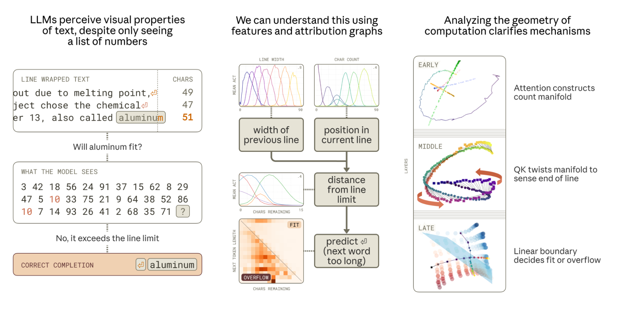
Introduction Intelligent systems need perception to understand, predict, and navigate their environment. These sensory capabilities reflect what's useful for survival in a specific environment: bats use echolocation, migratory birds sense magnetic fields, Arctic reindeer shift their UV vision seasonally. But when your world is made of text, what do you see? Language models encounter many text-based tasks that benefit from visual or spatial reasoning: parsing ASCII art, interpreting tables, or handling text wrapping constraints. Yet their only “sensory” input is a sequence of integers representing tokens. They must learn perceptual abilities from scratch, developing specialized mechanisms in the process. In this work, we investigate the mechanisms that enable Claude 3.5 Haiku to perform a natural perceptual task which is common in pretraining corpora and involves tracking position in a document. We find learned representations of position that are in some ways quite similar to the biological neurons found in mammals who perform analogous tasks (“place cells” and “boundary cells” in mice), but in other ways unique to the constraints of the residual stream in language models. We study these representations and find dual interpretations: we can understand them as a family of discrete features or as a one-dimensional “feature manifold”/“multidimensional feature” .All features have a magnitude dimension; so a discrete feature is a one-dimensional ray, and a one-dimensional feature manifold is the set of all scalings of that manifold, contracting to the origin. See What is a Linear Representation? What is a Multidimensional Feature? In the first interpretation, position is determined by which features activate and how strongly; in the latter interpretation, it's determined by angular movement on the feature manifold. Similarly, computation has two dual interpretations, as discrete circuits or geometric transformations. The task we study is linebreaking in fixed-width text. When training on source code, chat logs, email archives, scanned articles, or judicial rulings that have line width constraints, how does the model learn to predict when to break a line? Michaud et al. looked for “quanta” of model skills by clustering gradients . Their Figure 1 shows that predicting newlines in fixed-width text formed one of the top 400 clusters for the smallest model in the Pythia family, with 70m parameters. Human visual perception lets us do this almost completely subconsciously – when writing a birthday card, you can see when you are out of room on a line and need to begin the next – but language models see just a list of integers. In order to correctly predict the next token, in addition to selecting the next word, the model must somehow count the characters in the current line, subtract that from the line width constraint of the document, and compare the number of characters remaining to the length of the next word. As a concrete example, consider the below pair of prompts with an implicit 50-character line wrapping constraint.The wrapping constraint is implicit. Each newline gives a lower bound (the previous word did fit) and an upper bound (the next word did not). We do not nail down the extent to which the model performs optimal inference with respect to those constraints, rather focusing on how it approximately uses the length of each preceding line to determine whether to break the next. There are also many edge cases for handling tokenization and punctuation. A model could even attempt to infer whether the source document used a non-monospace font and then use the pixel count rather than the character count as a predictive signal! When the next word fits, the model says it; when it does not, the model breaks the line: To orient ourselves to the stages of the computation, we first studied the model using discrete dictionary features. In this frame, we can understand computation as an “attribution graph” where a cascade of features excite or inhibit each other.We actually first tried to use patching and probing without looking at the graph as a kind of methodological test of the utility of features, but did not make much progress. In hindsight, we were training probes for quantities different than the ones the model represents cleanly, e.g., a fusion of the current token position and the line width. The attribution graph shows how the model performs this task by combining features that represent different concepts it needs to track: Features for the current position in the line (the character count) as well as features for the total line width (the constraint) are computed by accumulating features for individual token lengths.The model then combines these two representations — current position and line width — to estimate the distance from the end of the line, leading to “characters remaining” features.Finally, the model uses this estimate of characters remaining along with features for the planned next word to determine if the next word will fit on the line or not. The attribution graph provides a kind of execution trace of the algorithm, showing on this prompt which variables are computed and from what. After finding large feature families involved in representing these quantities across a diverse dataset, we suspected a simpler lens might be provided in terms of lower-dimensional feature manifolds interacting geometrically. We found geometric perspectives on the following questions: How does the model represent different counts? The number of characters in a token, the number of characters in the current line, the overall line width constraint, and the number of characters remaining in the current line are each represented on 1-dimensional feature manifolds embedded with high curvature in low-dimensional subspaces of the residual stream. These manifolds have a dual interpretation in terms of discrete features, which tile the manifold in a canonical way, providing approximate local coordinates. Manifolds with similar geometry arise for a variety of ordinal concepts, and a ringing pattern we see in the embedded geometry in all these cases is optimal with respect to a simple physical model (§Representing Character Count).Ringing, in the manifold perspective, corresponds to interference in the feature superposition perspective. How does the model detect the boundary? To detect an approaching line boundary, the model must compare two quantities: the current character count and the line width. We find attention heads whose QK matrix rotates one counting manifold to align it with the other at a specific offset, creating a large inner product when the difference of the counts falls within a target range. Multiple heads with different offsets work together to precisely estimate the characters remaining (§Sensing the Line Boundary). How does the model know if the next word fits? The final decision — whether to predict a newline — requires combining the estimate of characters remaining with the length of the predicted next word. We discover that the model positions these counts on near-orthogonal subspaces, creating a geometric structure where the correct linebreak prediction is linearly separable (§Predicting the Newline). How does the model construct these curved geometries? The curvature in the character count representation manifold is produced by many attention heads working together, each contributing a piece of the overall curvature. This distributed algorithm is necessary because individual components cannot generate sufficient output variance to create the full representation (§A Distributed Character Counting Algorithm). We validate these interpretations through targeted interventions, ablations, and “visual illusions” — character sequences that hijack specific attention mechanisms to disrupt spatial perception (§Visual Illusions). Zooming out, we take several broader lessons from this mechanistic case study: When Models Manipulate Manifolds. For representing a scalar quantity (e.g., integer counts from 1 to N), it is inefficient to use N orthogonal dimensions, and not expressive enough to use just oneOrthogonal dimensions would also not be robust to estimation noise.. Instead models learn to represent these quantities on a feature manifold with intrinsic dimension 1 (the count) embedded in a subspace with extrinsic dimension 1 < d \ll N (e.g., ), in which the curve “ripples”. Such rippled manifolds optimally trade off capacity constraints (roughly, dimensionality) with maintaining the distinguishability of different scalar values (curvature). Our work demonstrates the intricate ways in which these manifolds can be manipulated to perform computation and show how this can require distributing computation across multiple model components. Duality of Features and Geometry. Dictionary features provide an unsupervised entry point for discovering mechanisms, and attribution graphs surface the important features for any particular prediction. Sometimes, discrete features (and their interactions) can be equivalently described using continuous feature manifolds (and their transformations). In cases where it is possible to explicitly parameterize the manifold (as with the various integer counts we study), we can directly study the geometry, making some operations clearer (e.g., boundary detection). But this approach is expensive in researcher time and potentially limited in scope: it's straightforward when studying known continuous variables but becomes difficult to execute correctly for more complex, difficult-to-parametrize concepts. Complexity Tax. While unsupervised discovery is a victory in and of itself, dictionary features fragment the model into a multitude of small pieces and interactions – a kind of complexity tax on the interpretation. In cases where a manifold parametrization exists, we can think of the geometric description as reducing this tax. In other cases, we will need additional tools to reduce the interpretation burden, like hierarchical representations or macroscopic structure in the global weights . We would be excited to see methods that extend the dictionary learning paradigm to unsupervised discovery of other kinds of geometric structures (e.g., those found in prior work ). Natural Tasks. The crispness of the representations and circuits we found was quite striking, and may be due to how well the model does the task. Linebreaking is an extremely natural behavior for a pretrained language model, and even tiny models are capable of it given enough context. Studying tasks which are natural for pretrained language models, instead of those of more theoretical interest to human investigators, may offer promising targets for finding general mechanisms. Preliminaries To enable systematic analysis, we created a synthetic dataset using a text corpus of diverse prose where we (1) stripped out all newlines and (2) reinserted newlines every k characters to the nearest word boundary \leq k for k=15,20,\ldots,150. As an example, here is the opening sentence of the Gettysburg Address, wrapped to k=40 characters, with the newlines shown explicitly. Claude 3.5 Haiku is able to adapt to the line length for every value of k, predicting newlines at the correct positions with high probability by the third line (see Appendix). All features in the main text of this paper are from a 10 million feature Weakly Causal Crosscoder (WCC) dictionary trained on Claude 3.5 Haiku. Feature activation values are normalized to their max throughout. Representing Character Count We define the line character count (or character count) at a given token in a prompt to be the total number of characters since the last newline, including the characters of the current token. A natural thing to check is if the model linearly represents the character count as a quantitative variable: that is, can we predict character count with high accuracy via linear regression on the residual stream? Yes: a linear probe fit on the residual stream after layer 1 has an R^2 of 0.985. This success does not mean, however, that the model actually represents the character count along a single line. Instead, we find a multidimensional representation of the character count that we will analyze from four perspectives: Sparse crosscoder features.Each feature has an encoder, which acts as a linear + (Jump)ReLU probe on the residual stream, and a decoder. Ten features f_1,\ldots,f_{10} are associated with line character count. The model's estimate of the character count, given a residual stream vector x, is summarized by the set of activities of each of the 10 features \{f_i(x)\}.A low-dimensional subspace.The model's estimate of the character count is summarized by the projection \pi(x) of x onto that subspace. Two datapoints have similar character counts if their projections are close in that subspace.A continuous 1-dimensional manifold contained in that low-dimensional subspace.The model's estimate of the character count is summarized by the nearest point on the manifold to the projection of x into the subspace, and its confidence in that estimate by the magnitude of \pi(x).A set of 150 logistic probes (corresponding to values of line character count from 1 to 150).The model's estimate of the character count is summarized by the probability distribution given by the softmax of the probe activities, softmax(Px). Each of these perspectives provides a complementary view of the same underlying object. The feature perspective is valuable for getting oriented, the subspace is perfect for causal intervention, the manifold is helpful for understanding how the representation is constructed and then manipulated to detect boundaries, and the logistic probes are useful for analyzing the OV and QK matrices of the individual attention heads involved. Character Count Features We begin with the features. In layers one and two, we found features that seemed to activate based on a token’s character position within a line. For example, in the attribution graph for the aluminum prompt, there were two features active on the final word “called” that seemed to fire when the line character count was between 35–55 and 45–65, respectively. To find more such features, we computed the mean activation of each feature binned by line character count. There were ten features with smooth profiles and large between-character-count variance, shown below: We find these features especially interesting as they are quite analogous to curve-detector features in vision models and place cells in biological brains . In all three of these cases, a continuous variable is represented by a collection of discrete elements that activate for particular value ranges. Moreover, we also observe dilation of the receptive fields (i.e., subsequent features activate over increasingly large character ranges) which is a common characteristic of biological perception of numbers (e.g., ). In the Appendix, we show these features are universal across dictionaries of different sizes, but that some feature splitting occurs with respect to the line width constraint. The Model Represents Character Count on a Continuous Manifold We observe that character count feature activations rise and fall at an offset, with two features being active at a time for most counts. This pattern suggests that the features are reconstructing a curved continuous manifold, locally parametrized by the activity of the two most active features. Given that their joint activation profiles follow a sinusoidal pattern, we expect reconstructions to lie on a curve between adjacent feature decoders. To visualize this, we first compute the average layer 2 residual stream for each value of line character count on our synthetic dataset. We compute the PCA of these 150 vectors, and find that the top 6 components capture 95% of the variance; we project data to that 6 dimensional subspace which we call the “character count subspace” (top 3 PCs on the left below, next 3 PCs on the right). We observe the data form a twisting curve, resembling a helix from the perspective of PCs 1–3 and a more complex twist from the perspective of PCs 4–6. We also reconstruct the residual stream for each datapoint using only the 10 character count features identified above, and compute the average reconstructed residual stream. We project the resulting curve, along with the feature decoders, into the same subspace. We find that the average line character count vectors are quite closely approximated by the feature reconstruction, though with mild kinks near the feature vectors themselves, reminiscent of a spline approximation of a smooth curve. While the 10 feature vectors discretize the curve, interpolating between the 2–3 neighboring features which are active at a time allows for a high-quality reconstruction of 150 data points. Validation: The Character Count Subspace is Causal To validate our interpretation of the character count subspace, we perform a coarse-grained ablation and a fine-grained intervention. Ablation Experiment. For our ablation experiment, we zero ablate (from a single early layer) a k-dimensional subspace corresponding to the top k principal components of the per–character count mean activations and compare to a baseline of ablating a random k-dimensional subspace. Below we measure the loss effect, broken down by newlines and nonnewlines.Note, in general one should not assume that a subspace spanned by features (or a PCA) is dedicated to those features because it could be in superposition with many other features. However, because in this case the character count subspace is densely active (and therefore less amenable to being in superposition), this experimental design is more justified. Intervention Experiment. As a more surgical intervention, we perform an experiment to modify the perceived character count at the end of the aluminum prompt (originally 42 characters). Specifically, we sweep over character counts c, and substitute the mean activation across all tokens in our dataset with count c. That is, a_{\text{patched}} = a_{\text{original}} - \mu_{\text{original}} + \mu_{c} for activation a and average activation matrix \mu. We perform this intervention for three adjacent early layers and the last two tokens for both the entire mean vector and within the 6 dimensional PCA space of the mean vectors. The attribution graph has several positional features and edges on both the last token (“called”) as well as the second-to-last token (“also”). We change the “also” count representation to be 6 characters prior to that for the final token, to maintain consistency. The Probe Perspective We also train supervised logistic regression probes to predict character count.as a 150-way multiclass classification problem Probes trained after layer 1 achieve a root mean squared error of 5, indicating some intrinsic noise in the character count representation — which is consistent with our features having relatively wide receptive fields. Performing PCA on the 150 probe weight vectors, we find that 6 components capture 82% of the variance. When we look at the average responses of each probe to tokens with different line character counts, we see a striking pattern. In addition to a diagonal band (probes, like the sparse features, have increasingly wide receptive fields), we see two faint off-diagonal bands on each side! The response curve of each probe is not monotonically decreasing away from its max, but rebounds. This “ringing” turns out to be a natural consequence of embedding a “rippled” manifold into low dimensions. Rippled Representations are Optimal We note that the cosine similarities of the mean activation vector (which form the helix-like curve visualized in PCA space above), the linear probe vectors, and feature decoder vectors all exhibit similar ringing patterns to the above figure.We use the term “ringing” in the sense of signal processing, a transient oscillation in response to a sharp peak, such as in the Gibbs Phenomenon). Note that not only are neighboring features not orthogonal, features further away have negative similarities, and then those even further away have positive ones again. This structure turns out to be a natural consequence of having the desired pattern of similarity, trivially achievable in 150 dimensions, projected down to low dimensions. As a toy model of this, suppose that we wish to have a discretized circle's worth of unit vectors, each similar to its neighbors but orthogonal to those further away. This can be realized by a symmetric set of unit vectors in 150 dimensions with cosine similarity matrix X pictured below (left). Projecting this to its top 5 eigenvectors yields a 5-dimensional embedding of the same vectors with cosine similarity matrix (below right) exhibiting ringing. We also plot the curve these vectors form in the top 3 eigenvectors. We can think of the original 150-dimensional embedding of the circle as being highly curved, and the resulting 5-dimensional embedding as retaining as much of that curvature as possible. This manifests as ripples in the embedding of the circle when viewed in a 3D projection. A relationship of this construction to Fourier features is discussed in the appendix. Alternatively, one can view the ringing from the perspective of sparse feature decoders as a kind of interference weight . With no capacity constraints, the model might use orthogonal vectors to represent the quantitative response of each feature, with its own receptive field, to the input data. Forced to put them into lower dimensional superposition, the similarity matrix picks up both a wider diagonal stripe and the upper/lower diagonal ringing stripes. Finally, we also construct a simple physical model showing that the rippling and ringing arise even when the solution is found dynamically, whenever many vectors are packed into a small number of dimensions. Below, we show the result of a simulation in which 100 points confined to a 6-dimensional hypersphere are subjected to attractive forces to their 6 closest neighbors on each side (matching the RMSE error of our probes) and repulsive forces to all other points. (To avoid boundary conditions, we use the topology of a circle instead of an interval.) On the right below is a heatmap exhibiting two rings, and on the left is a 3-dimensional projection of the 6-dimensional curve. This simulation is interactive, and the reader is encouraged to experiment with reinitializing the points (↺), switching the ambient dimension, and modifying the width of the attractive zone. Decreasing the attractive zone or increasing the embedding dimension both increase curvature (and the amount of ringing), and vice versa.The simulation can sometimes find itself in local minima. Increasing the width of the attractive zone before decreasing it again usually solves this issue. As the number of points on the curve grows and the attractive zone width shrinks (in relative terms), the curvature grows quite extreme, approaching a space-filling curve in the limit. Of particular interest is the result from setting the ambient dimension to 3Optimization in dimension 3, unlike in higher dimensions, admits bad local minima, because a generic curve on the surface of a sphere self-intersects. To avoid this, either increase the zone width until you get a great circle, then decrease it, or do the optimization in 4D, then select 3D.: the result is a curve similar to the seams of a baseball (below left, circle), which matches the topology observed for three intrinsically one-dimensional phenomena observed in , of colors by hue, dates of the year, and years of the 20th century (which also exhibit dilation). Similar ripples were predicted to occur by Olah and then observed by Gorton in curve detector features in Inception v1. One of the earliest observations of ringing in a cosine similarity plot and rippled spiral/helix shape in a low-dimensional embedding was of the learned positional embeddings of tokens in GPT2 . We also find similar structure in other representations, which we study in More Sensory and Counting Representations in the appendix. Sensing the Line Boundary We now study how the character counting representations are used to determine if the current line of text is approaching the line boundary. To detect the line boundary, the model needs to (1) determine the overall line width constraint and (2) compare the current character count with the line width to calculate the characters remaining. Twisting with QK We find that newline tokens have their own dedicated character counting features that activate based on the width of the line, counting the number of characters between adjacent newlines. To better understand how these representations are related, we train 150 probes for each possible value of “Line Width” like we did for “Character Count”. Using the attribution graph, we identify an attention head which activates boundary detection features. We visualize both sets of counting representations directly using the first 3 components of their joint PCA in the residual stream (left) and in the reduced QK space of this boundary head (right).Specifically we multiply the line width probes through W_K and the character count probes through W_Q, and plot the points in the 3D PCA basis of their joint embedding. We find that this attention head “twists” the character count manifold such that character count i is aligned with line width k=i+\epsilon. This causes the head to attend to the newline when the character count is just a bit less than the line width, thereby indicating that the boundary is approaching. This algorithm is quite general, and enables this head to detect approaching line boundaries for arbitrary line widths!This algorithm also generalizes to arbitrary kinds of separators (e.g., double newlines or pipes), as the QK circuit can handle the positional offset independently of the OV circuit copying the separator type. This plot shows that In the residual stream, probes for character count i are maximally aligned with probes line width probes k when i=k, but are not highly aligned in absolute terms – the maximum cosine sim is ~0.25. In the QK space of the boundary head, the probes are maximally aligned on the offdiagonal i }} ;| || `, @@. We further analyzed the extent to which there was a relationship between ‘distraction’ of the important attention heads and the impact on the newline prediction. Indeed we found that many of the sequences with potent modulation of newline probability––and especially code-related character pairs––also exhibited substantial modulation of attention patterns. While in the aluminum prompt the task is implicit, this illusion generalizes to settings where the comparison task is made explicit. These direct comparisons are perhaps more analogous to the Ponzo, Sander, and Müller-Lyer illusions, where the perception and comparison is more direct. These effects are robust to multiple choice orderings. Moreover, if the length of the text following the @@ exceeds that of the alternative choice, the alternative choice is selected as being shorter. While we are not claiming any direct analogy between illusions of human visual perception and this alteration of line character count estimates, the parallels are suggestive. In both cases we can see the broader phenomena of contextual cues, and the application of learned priors about those cues, modulating estimates of object properties of entities. In the human case, priors such as three-dimensional perspective can influence perception of object size, or color constancy can influence estimates of luminance (such as in the checker shadow illusion). Here, one possible interpretation of our results is that mis-application of a learned prior, including the role of cues such as @@ in git diffs, can also modulate estimates of properties such as line length. Related Work Objective. This work is at the intersection of LLM “biology” (making empirical observations about what is going on inside models; e.g. ) and low level reverse engineering of neural networks (attempting to fully characterize an algorithm or mechanism; e.g. ). Methodologically, our work makes heavy use of attribution graphs with QK attributions built on top of crosscoders . Linebreaking. Michaud et al. identified linebreaking in fixed-width text as one of the top 400 “quanta” of model behavior in the smallest model (70m parameters) in the Pythia suite. Position. Prior interpretability work on positional mechanism has largely focused on token position (e.g., ). These works have shown that there exist MLP neurons , SAE features , and learned position embeddings with periodic structure encoding absolute token position. Our work illustrates how a model might also want to construct non-token based position schemes that are more natural for many downstream prediction tasks. Others have also studied, even going back to LSTMs, the existence of mechanisms in language models for controlling the length of output responses , as well as performed more theoretical analyses of the space of counting algorithms . Geometry and Feature Manifolds. Beyond position, there has been extensive work in understanding the geometric representation of numbers, especially in toy models (e.g., ) and in the context of arithmetic in LLMs (e.g., ). Collectively, these works have shown that both real LLMs and toy transformers learn periodic representations , with numbers arranged in a helix to enable certain matrix multiplication based addition algorithms , and that these representations are provably optimal in certain settings . In our context, we similarly observe helical representations , numeric dilation , and distributed algorithms across components that collectively implement a correct computation . Multidimensional features with clear geometric structure have been found in more natural contexts , like in the representation and computation of certain ordinal relationships (e.g., months of the year). In vision models, curve detector neurons and features have been especially well studied and closely resemble the kind of discretization we observe with the families of character counting features. Many other topics have received interpretability analysis of the underlying geometry, such as grammatical relations , multilingual representations , truth , binding , refusal , features , and hierarchy , though more conceptual research is needed . Perhaps most relevant is recent work from Modell et al. , who provide a more formal notion of a feature manifold, and propose that cosine similarity encodes the intrinsic geometry of features. When testing their theory, they observe highly structured and interpretable data manifolds that have ripples and dilation, similar to our counting manifolds. These observations raise a methodological challenge in how to best capture data with different structure (see e.g. ), but also the exciting hypothesis that many naturally continuous variables (e.g., ) exist in more organized manifolds. Biological Analogues. The geometric and algorithmic patterns we observe have suggestive parallels to perception in biological neural systems. Our character count features are analogous to place cells on a 1-D track and our boundary detecting features are analogous to boundary cells . These features exhibit dilation—representing increasingly large character counts activating over increasingly large ranges—mirroring the dilation of number representations in biological brains . Moreover, the organization of the features on a low dimensional manifold is an instance of a common motif in biological cognition (e.g., ). While the analogies are not perfect, we suspect that there is still fruitful conceptual overlap from increased collaboration between neuroscience and interpretability . In this paper, we studied the steps involved in a large model performing a naturalistic behavior. The linebreaking task, frequently encountered in training, requires the model to represent and compute a number of scalar quantities involving position in character count units that are not explicit in its input or outputTokens do not come annotated with character counts, and there are no vertical bars on the page showing the line width., then integrate those values with the outputs of complex semantic circuits (that predict the next proper word) to predict the next token. We found sparse features corresponding to each important step of the computation, and for those steps involving scalar quantities, we were able to find a geometric description that significantly simplified the interpretation of the algorithm used by the model. We now reflect on what we learned from that process: Naturalistic Behavior and Sensory Processing. Deep mechanistic case studies benefit from choosing behaviors that the model performs consistently well, as these are more likely to have crisper mechanisms. This means prioritizing tasks that are natural in pretraining over tasks that seem natural to human investigators, and ideally, that are easily supervisable. As in biological neuroscience, perceptual tasks are often both natural and easy to supervise for interpretability (e.g., it is easy to modify the input in a programmatic way). Although we sometimes describe the early layers of language models as responsible for “detokenizing” the input , it is perhaps more evocative to think of this as perception. The beginning of the model is really responsible for seeing the input, and much of the early circuitry is in service of sensing or perceiving the text similar to how early layers in vision models implement low level perception . The Utility of Geometry. Many of the representations and computations we studied had elegant geometric interpretations. For example, the counting manifolds are the result of an optimal tradeoff between capacity and resolution, with deep connections to space-filling curves and Fourier features. The boundary head twist was especially beautiful, and after discovering one such head, we were able to correctly predict that there would need to be additional heads to provide curvature in the output. The distributed character counting algorithm was more complex, but we were still able to clarify our view by studying linear actions on these manifolds. For other computations, like the final breaking decision, the linear separation was clearly a part of the story but there must be some additional complexity we were not able to see yet to handle multitoken outputs. For the more semantic operations, we purely relied on the feature view. Of course, describing any behavior in full is immensely complicated, and there is a long list of possible subtleties we did not study: how the model accounts for uncertainty in its counting, its mechanism for estimating the line width given multiple prior lines of text, how it adapts to documents with variable line width, how it handles multiple plausible output tokens of different lengths or multitoken words, or various special cases (e.g., a LaTeX \footnote{} or a markdown link). For the inspired, we share transcoder attribution graphs for a fixed-width line break prompt on Gemma 2 2B and Qwen 3 4B, using the new neuronpedia interactive interface. Unsupervised Discovery It likely would not have been possible to develop this clarity if it were not for the unsupervised sparse features. In fact, when we started this project, we attempted to just probe and patch our way to understanding, but this turned out poorly. Specifically, we did not understand what we were looking for (e.g. we didn’t know to distinguish line width vs. character count), where to look for it (e.g., we didn’t expect line width to only be represented on the newline), or how to look for it (we started by training 1-D linear regression probes). However, after identifying some relevant features but before spending substantial effort systematically characterizing their activity profiles, we were also confused by what they were representing. We saw dozens of features that were vaguely about newlines and linebroken text, but their differences were not obvious from flipping through the activating examples. Only after we tested these features on synthetic datasets did their role in the graph and the underlying computation become clear. We suspect better automatic labels enhanced with agentic workflows would accelerate this work, especially in less verifiable domains. Feature-Manifold Duality. The discrete feature and geometric feature-manifold perspectives offer dual lenses on the same underlying object. For example, in this work the model's representation of character count can be completely described (modulo reconstruction error) by the activities of the features we identified, where the action of the boundary heads is described by virtual weights that expand out the feature interactions via attention head matrices. The same character count representation can be described by a 1-dimensional feature manifold – a curve in the residual stream parametrized by the character count variable – where linear action of the boundary heads is described by continuous “twisting” of the manifold. In general, geometric structures learned by the model will likely admit both global parametrizations and local discrete approximations. The Complexity Tax. Despite this duality, the descriptions produced by the two perspectives differ in their simplicity. The discrete features shatter the model into many pieces, producing a complex understanding of the computation. This seems like a general lesson. It seems like discrete features and attribution graphs may provide a true description of model computation, which can be found in an automated way using dictionary learning. Getting any true, understandable description of the computation is a very non-trivial victory! However, if we stop there, and don't understand additional structure which is present, we pay a complexity tax, where we understand things in a needlessly complicated way. In the line breaking problem, constructing the manifold paid down this tax, but one could imagine other ways of reducing the interpretation burden. A Call for Methodology. Armed with our feature understanding, we were able to directly search for the relevant geometric structures. This was an existence proof more than a general recipe, and we need methods that can automatically surface simpler structures to pay down the complexity tax. In our setting, this meant studying feature manifolds, and it would be nice to see unsupervised approaches to detecting them. In other cases we will need yet other tools to reduce the interpretation burden, like finding hierarchical representations or macroscopic structure in the global weights . A Call for Biology. The model must perform other elegant computations. We can find these by starting with a specific task the model performs well, study this from multiple perspectives, develop methodology to answer the remaining questions, and relentlessly attempt to simplify our explanations. Because the investigation is grounded in specific examples of a behavior, it provides a fast feedback loop, can shed light on weaknesses of existing methods and inspire new ones, and can sharpen our conceptual language for understanding neural networks. We would be excited to see more deep case studies that adopt this approach.